Data Mining Twitter Using R: A guide for the Very Online

By Tony Damiano (@tony_damiano)

I Just Wanted to Learn Data Science

Thursday, Nov 15, 2018, Washington Examiner reporter Eddie Scarry broke the internet worse than Kim Kardashian ever could. In a tweet for the ages, the conservative skeezeball best known for taking unsuspecting foot pics of random women at restaurants , against all better advice and decency decided to dress down newly elected socialist congresswoman from New York Alexandria Ocasio-Cortez.

 
bad-tweet.png


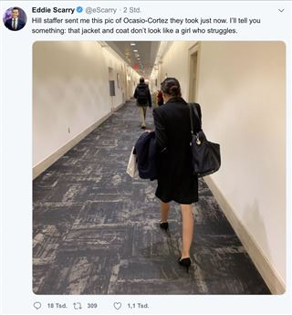
"This is our balloon boy"

I'll take you inside our dm for the play by play. The reaction to Eddie's bad tweet started slowly at first but snowballed as the afternoon progressed.

 
dm1.png
dm2.png
 

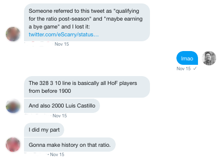
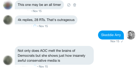
After a while, the replies kept coming and it wasn't clear Mr. Scarry would make it through the night.

 
dm5.png
dm3.png
 

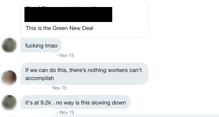
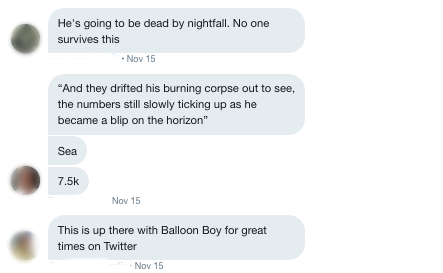
By the time the things got rolling, there were over 10,000 replies before he deleted the tweet. Despite calling it a day, he decided to tweet through it. Each of his responses spawned its own mini-ratio in a cascading series of ratios that filled the internet (or at least my dm) with unadulterated glee.


I had been wanting to learn how to gather twitter data for quite some time and instead of practicing on something useful, I decided to examine the beauty of Mr. Scarry's ratio for the ages.

The following contains the analysis I performed using a sample of Mr. Scarry's mentions that day interspersed with R code so hopefully my wasted time can provide some social benefit to several nerds who may eventually read this.

Getting started

Setting Up a Twitter App

Since you're reading a post called data mining for the "very online" I'm going to assume you have a twitter account and are somewhat familiar with this hell site. You will, however, need to create an app and generate tokens which will allow you to access Twitter data from their API.

For this analysis, I used the rtweet  package created by Professor Michael W. Kearney at the University of Missouri. Professor Kearney has a great guide to get you started.

Set up a Twitter App

SIDENOTE: If you are new to R, I would highly recommend R for Data Science by Garrett Grolemund and Hadley Wickham.

After I set up the app, I entered the tokens generated into rtweet. I also loaded a few other packages to help with data analysis and cleaning.

if (!require(pacman)) install.packages('pacman')
library(pacman)
p_load(tidyverse,  # Suite of tools for data analysis using "tidy" framework                                                     rtweet,     # Access twitter data                                                                                           tidytext,   # Tools for text analysis                                                                                       maps        # Map data                                                                                                      )
create_token(consumer_key = "Your-Token-Here",                                                                              consumer_secret = "Your-Token-Here",                                                                                        access_token  = "Your-Token-Here",                                                                                          access_secret = "Your-Token-Here")

The main function rtweet uses to gather tweet data is search_tweets.

For this analysis, I queried the Twitter API for tweets containing Mr. Scarry's twitter handle @eScarry" on the date of the incident (I performed this query the night of the 15th, your results if you performed the same query may look different compared to mine).

NOTE: Twitter limits queries to 18,000 tweets per 15 minutes so setting retryonratelimit = T would allow you to see the full extent of the damage. Did I decide to search for more, because why not?

scarry_menchies <- search_tweets(q, n = 20000,                                                                                                               retryonratelimit = TRUE,                                                                                                    include_rts = FALSE,                                                                                                        since  = "2018-11-15")

Plan for 10-15 minutes to download a larger dataset like this (see here for more info on the Twitter API). rtweet also has to parse the data from JSON to an R data.frame or tibble which takes some time too.

The Data

Twitter's API is rich and includes a wealth of information, 88 columns in total. To think, your hours and hours of shit posting can be summed up such a beautiful tabular format! Here's a look at the first 10 columns. The first interesting thing to note is that I ended up with close to double the number of tweets I requested (my guess is since I set retryonratelimit = T  the query stopped after hitting the rate limit twice). Just more data for us!

scarry_menchies %>%                                                                                                           select(1:10) %>%                                                                                                            glimpse()

## Observations: 34,995                                                                                                     ## Variables: 10                                                                                                            ## $ user_id              <chr> "131173072", "21507325",                                                                    "103414773200340...                                                                                                         ## $ status_id            <chr> "1063269890637918208",                                                                      "10632698846233149...                                                                                                       ## $ created_at           <dttm> 2018-11-16 03:17:51, 2018-11-16                                                            03:17:49...                                                                                                                 ## $ screen_name          <chr> "artisgoodck", "kevinkam", "K4Mst3",                                                        "Was...                                                                                                                     ## $ text                 <chr> "@Ocasio2018 @eScarry Omg. Some of my                                                       bes...                                                                                                                      ## $ source               <chr> "Twitter for iPhone", "Twitter for                                                          Androi...                                                                                                                   ## $ display_text_width   <dbl> 119, 77, 57, 21, 31, 20, 67, 0, 0, 0, 0,                                                    ...                                                                                                                         ## $ reply_to_status_id   <chr> "1063240055236501505",                                                                      "40823788385036288...                                                                                                       ## $ reply_to_user_id     <chr> "138203134", "18155174", "18155174",                                                        "181...                                                                                                                     ## $ reply_to_screen_name <chr> "Ocasio2018", "eScarry", "eScarry",                                                         "eSca...

A quick look reveals the range of timestamps of tweets I collected shows the replies I queried were written between 4:06 pm CST and 9:17 pm CST on November 15th. That's 120 tweets per minute! Tough look for my guy Eddie.

min(scarry_menchies$created_at)                                                                                             ## [1] "2018-11-15 22:06:51 UTC"

max(scarry_menchies$created_at)                                                                                             ## [1] "2018-11-16 03:17:51 UTC"


An international phenomenon

Before I did any more intense cleaning, I decided to take a look at the geographic distribution of the mentions. Using lat_lng  from rtweet and simple mapping capabilities of ggplot2, we can see The Bad Tweet was truly an international phenomenon. Though only a small sample of tweets were geotagged (n = 1087), we can see a multitude of tweets coming from outside of the US including a smattering across Europe, Canada, Australia and at least one brave soul in the United Arab Emirates.

world <- ggplot2::map_data("world")                                                                                         sm_coords <- lat_lng(scarry_menchies)                                                                                       ggplot() +                                                                                                                   geom_polygon(data = world, aes(x = long, y = lat, group = group)) +                                                         geom_point(data = sm_coords, aes(x = lng, y = lat), color = "#01FF70",                                                     size = 0.5) +                                                                                                                coord_quickmap() +                                                                                                          guides(fill = FALSE) +                                                                                                      labs(title = "    Geographic Distribution of the mentions of @eScarry's                                                    Bad Tweet",                                                                                                                        caption = "@tony_damiano") +                                                                                           theme_void()                                                                                                              
 
unnamed-chunk-5-1.png
 

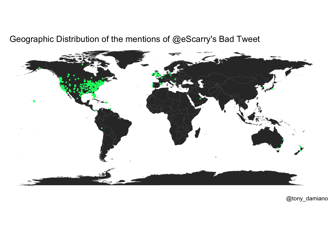
What do these beautiful menchies actually say?

Now everybody's favorite part. Data cleaning! Despite the tweet being gone, its unique ID survives! We can filter our data set to include just replies to Mr. Scarry's bad tweet if we were so inclined, but as I mentioned earlier, we'll use all of the data from the menchies we gathered.

# Not run for this analysis                                                                                                 scarry_menchies_tweet <- scarry_menchies %>%                                                                                  filter(reply_to_status_id == "1063183409458102272") #the bad tweet

Tweets contain a lot of information that isn't text -- Specifically, twitter usernames and URLs. I used regular expressions filter out some of the noise. For those new to regular expressions, they are  a humanly incomprehensible and tortuous way to parse text for specific patterns within text strings. There are those brave enough to learn its secrets, but I'm content searching Stack Exchange. No reason to reinvent the wheel.

In this next step, I used the tidytext package to remove all punctuation, make all words lower-case and remove common words like "it", "is", "as", and so forth. The key function I used was the unnest_tokens function. unnest_tokens converts each word to lower case and breaks each word into its own line giving us one very very long, 1 x n-words dataset. I removed the HTML and twitter handles, then removed common english words with included "stop_words" list.

#Remove urls                                                                                                                text <- scarry_menchies$text %>%                                                                                              gsub("http.*", "", .)                                                                                                                                                                                                                                 #Remove Twitter Handlestext <-                                                                                              text %>%                                                                                                                      gsub("(^|[^@\\w])@(\\w{1,15})\\b", "", .) %>%                                                                               as_tibble() %>%                                                                                                             unnest_tokens(word, value)                                                                                                                                                                                                                            # Remove stop words (common English words)                                                                                  data("stop_words"                                                                                                                                                                                                                                       cleaned <- text %>%                                                                                                           anti_join(stop_words)

Top 20 Words

As a first step, I plotted the most frequently used 20 words from my sample of Eddie’s mentions. Many of these are to be expected given the content of the original tweet (words like "clothes", "jacket" etc.), however, the internet came through with "ratio" as the top word in all of Me. Scarry's mentions and "creepy" also making it into the top 10.

#Top 20 Words                                                                                                               top20 <- cleaned %>%                                                                                                          count(word, sort = TRUE) %>%                                                                                                top_n(20) %>%                                                                                                               mutate(word = reorder(word, n)) %>%                                                                                         ggplot(aes(x = word, y = n)) +                                                                                              geom_col() +                                                                                                                coord_flip() +                                                                                                              labs(y = "Counts",                                                                                                               x = "",                                                                                                                     title = "Top 20 unique words found in the mentions of                                                                       @eScarry's Bad Tweet",                                                                                                      caption = "@tony_damiano") +                                                                                           theme_minimal() +                                                                                                           theme(axis.text.y = element_text(size = 12))
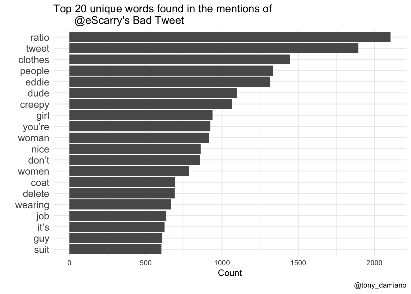
 
unnamed-chunk-8-1.png
 

N-Grams

tidytext is a flexible package and we can expand our frequency analysis and look at phrases too. Below is the same analysis as above except I told tidytext to find all two-word phrases. A lot of ratio talk going on.

ngram2 <- text %>%                                                                                                            unnest_tokens(paired_words, word, token = "ngrams", n = 2) %>%                                                              count(paired_words, sort = T) %>%                                                                                           top_n(20) 
ngram2 %>%                                                                                                                    mutate(paired_words = reorder(paired_words, n)) %>%                                                                         ggplot(aes(x = paired_words, y = n)) +                                                                                      geom_col() +                                                                                                                coord_flip() +                                                                                                              labs(y = "Count",                                                                                                                x = "",                                                                                                                     title = "Top 20 two-word phrases found in the mentions of                                                                   @eScarry's Bad Tweet",                                                                                                      caption = "@tony_damiano") +                                                                                           theme_minimal() +                                                                                                           theme(text = element_text(size=14))
 
unnamed-chunk-9-1.png
 

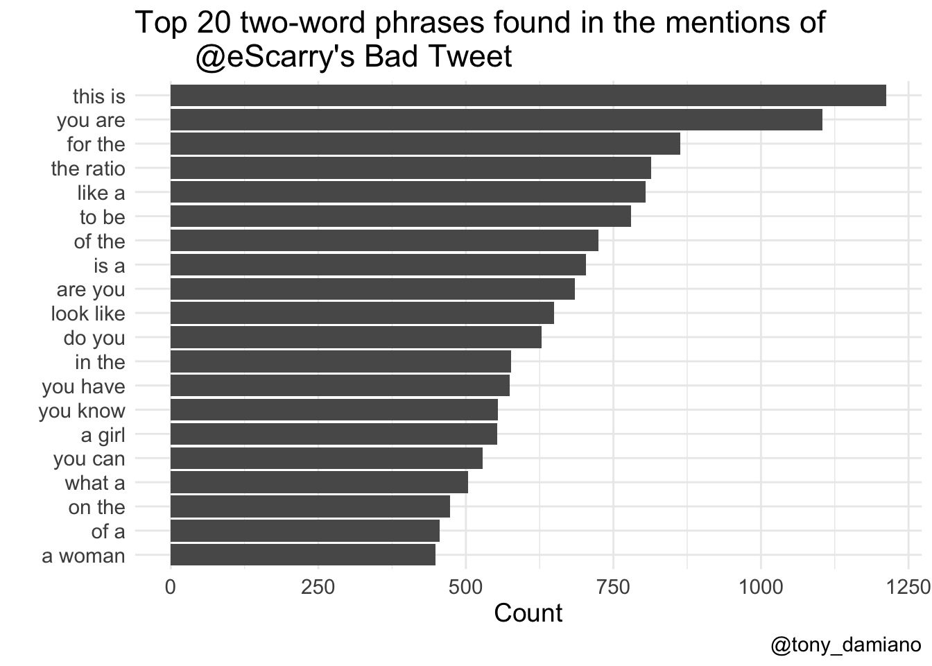
Just Here for the Ratio

I performed the same analysis with three and four-word phrases (not pictured here), but the breakthrough happened once I queried five-word phrases. The number one five-word phrase in the mentions of Eddie's bad tweet was "just here for the ratio.”

ngram5 <- text %>%                                                                                                            unnest_tokens(n_words, word, token = "ngrams", n = 5) %>%                                                                   count(n_words, sort = T) %>%                                                                                                top_n(10)
ngram5 %>%                                                                                                                    mutate(n_words = reorder(n_words, n)) %>%                                                                                   ggplot(aes(x = n_words, y = n)) +                                                                                           geom_col() +                                                                                                                coord_flip() +                                                                                                              labs(y = "Count",                                                                                                                x = "",                                                                                                                     title = "Top 10 five-word phrases found in the mentions of                                                                  @eScarry's Bad Tweet",                                                                                                      caption = "@tony_damiano") +                                                                                           theme_minimal() +                                                                                                           theme(text = element_text(size=12))
 
unnamed-chunk-10-1.png
chef.png
 

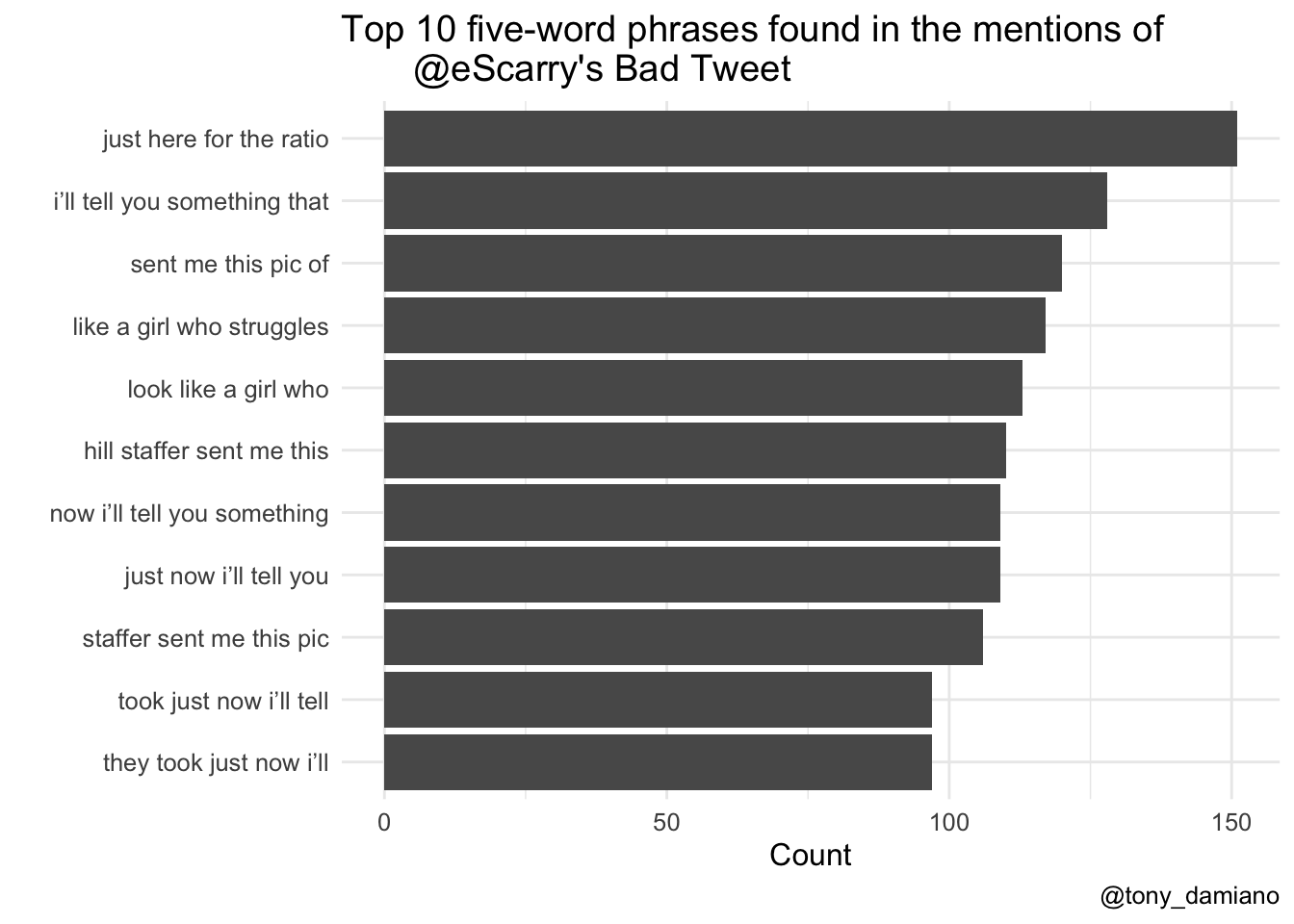
Sometimes being on Twitter pays off.

Data Science Binch!

Lastly, as a measure of the density of weird left twitter's engagement, I did a query using common weird left twitter phrases including "binch", "corncob" and "chief.”

#Remove Twitter Handles                                                                                                     text <- text %>%                                                                                                              gsub("(^|[^@\\w])@(\\w{1,15})\\b", "", .) %>%                                                                               as_tibble() %>%                                                                                                             unnest_tokens(word, value) 
# Remove stop words (common english words)                                                                                  data("stop_words")
cleaned <- text %>%                                                                                                         anti_join(stop_words)
cleaned %>%                                                                                                                   count(word, sort = TRUE) %>%                                                                                                filter(str_detect(word, "binch") |                                                                                                 str_detect(word, "corncob") |                                                                                               str_detect(word, "chief")                                                                                                   ) %>%                                                                                                                mutate(word = reorder(word, n)) %>%                                                                                         ggplot(aes(x = word, y = n)) +                                                                                              scale_y_continuous(breaks = scales::pretty_breaks()) + #for integer values on count axis                                            geom_col() +                                                                                                                xlab(NULL) +                                                                                                                coord_flip() +                                                                                                              labs(y = "Count",                                                                                                                x = "",                                                                                                                     title = "Words in the mentions of @eScarry's bad tweet containing                                                           'binch', 'corncob' and 'chief'",                                                                                            caption = "@tony_damiano")
 
unnamed-chunk-11-1.png
 

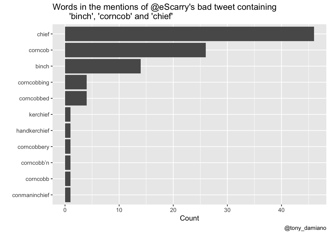
I found "chief" to be the most popular word in this query (n = 46) followed by "corncob" (n = 26) and "binch" (n = 14). There were some lovely riffs on corncob that are worth mentioning including as a present participle "corncobbing", past participle "corncobbed", vernacular present participle "corncob'n" (something you do with the fella's on a lazy afternoon) and my personal favorite - "corncobbery" which is a noun that I define the behavior of an internet buffoon who refuses to log off.

Conclusion

My conclusions from this analysis are threefold:
 1. Eddie Scarry made a really bad tweet
 2. Twitter responded in magnificent fashion
 3. I can leverage my onlineness for good, not just shitposting

Raw source code and data from this analysis are available on my github here.


Tony Damiano (@tony_damiano) is a PhD candidate at the University of Minnesota studying housing policy, race, neighborhoods, and inequality. He is passionate about housing justice, data democracy, and Italian food.

Guest User